Introduction
Suppose you have reason to believe that a biomarker signal could precede a clinical diagnosis, leading to earlier and better intervention. You have a large collection of candidate biomarkers, and you think possibly a small number of them could form the basis of this predictive signal. You assemble a collection of clinical subjects for whom you take blood samples repeatedly over time. Some of them go on to be diagnosed; others never do, and leave the study.
This is almost, but not quite, a biomarker discovery / classification problem. Analysts have an enormous bank of biomarker discovery and classification tools, so we’re inclined to turn to those. But applying stock classification methods is forcing a round peg into a square hole: there is a resemblance, yet there are key differences, as I explain in the next section.
The biggest difference is that classification is appropriate when there is a clear, well-defined time to make a classification decision (or to decide that the case isn’t clear). Monitoring is appropriate when the question of when to make a call is very much in play.
I find that for the monitoring problem, there is not a tool that estimates coefficients straightforwardly, the way logistic regression does in the binary classification context. My proposal offers this; accordingly I call it “Monitoring Regression”.
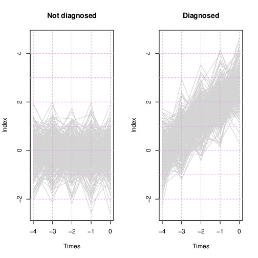
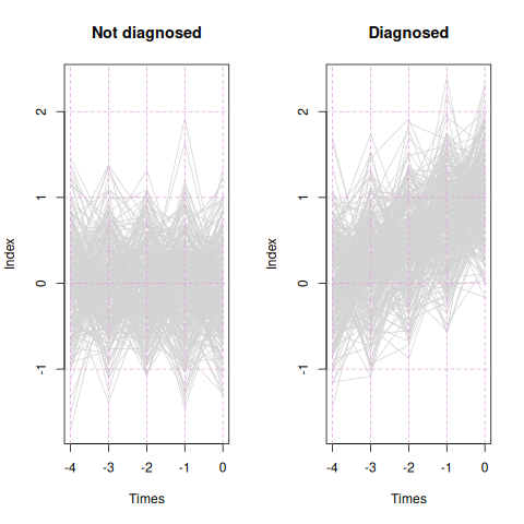
Here’s a teaser for the remainder of the essay: I simulated 600 hypothetical subjects with 40 biomarkers, each subject observed at five time points. 300 patients were diagnosed at the last time point, while the other 300 were not. Four of the 40 variables were informative for predicting the diagnosis, while the other 36 were not. The Monitoring Regression process I describe below selected the four informative variables, neglected the rest, and estimated a linear combination of the four, which Figure 1 shows for each patient, separately for the diagnosed and not-diagnosed groups.
This essay is a high-level description intended for a non-statistical, yet interested, audience. I plan to submit a more detailed article for publication.
It would be grand to try out the method on a real-world example. If you have a suitable example, I’d be happy to do carry out regression fitting, and propose a follow-up monitoring program, for no fee, if I can use the example in publication. Some obscuring of data and identifying aspects of the problem so as to not give away key secrets are permissible. If interested, please contact me.
Related applications
An application related to biomarker discovery for diagnostic monitoring is monitoring signals over time, such as EKG’s or EEG’s. This would probably require some pre-processing or extension, such as applying a wavelet transform or fitting a neural net, or fitting a neural net to wavelet coefficients.
Another area is mining streams of telemetry sent by electro-mechanical systems in order to develop a monitoring regime to identify likely failures as early as possible.
The right method for the problem
The classification task, in clinical application, uses biomarker(s) to classify patients, usually as “Positive” or “Negative”. However, in many cases what the analyst truly desires is to find measurements that may be predictive when monitored over time. The monitoring and the classification contexts are distinct.
In a classification problem, data from each patient is complete and mature at a designated point in the patient’s time course (modulo some data imputation in real applications). We train a model to generate class probabilities, which can then support decisions of “Positive”, “Negative”, or “Uncertain”. (In some cases, the system doesn’t provide probabilities but simply makes class decisions directly.)
In the monitoring context, we have data available at multiple time points per subject, and at each time point the monitoring system determines “Positive” or “Continue monitoring”. It resembles classification except that determining the time of call is a critical aspect of the problem; most likely, we could make a call earlier, but less accurately; or later, and more accurately. Perhaps some patients could be called with high confidence at an early time, while others gain no time advantage at all.
Time alignment
Furthermore, the two contexts differ in time alignment. In classification, we assume that the question of when to attempt classification has already been answered. If data from prior time points is to be included in the classification, we assume that these data are comparable and complete. If time-series signals are used, they’ve been appropriately aligned. And so on.
Generally there needs to be a universal definition of “time zero”, relative to which all other times are expressed, either before or after. In some cases time zero is the time of entry to the study. However, if patients can be tracked for an indefinite and variable period of time, after which a diagnosis is made, then the time of diagnosis is the relevant benchmark, and we ask, “By how much time preceding the diagnosis can we make a clinically valuable call?” However, the benchmark of diagnosis time is not available for the patients who were never diagnosed. To apply classification methods, we have to come up with some benchmark for this group. Perhaps we choose a time randomly. Perhaps any time is as good as any other, or perhaps not. It’s problem-dependent. At any rate, there is no clearly appropriate time benchmark when a patient was never diagnosed, yet we must “make up something”.
Tendency to use classification methods
If a patient in a well-defined context appears in a clinical setting and the physician must make a decision at that time, then classification may be the appropriate tool. However, often the physician observes the patient over time, taking measurements in sequence, and has to determine when enough evidence has accumulated to justify intervention. This paradigm is better described by the monitoring context.
Even though many health decision-making questions better fit the monitoring characterization, analysts pursuing empirical methods almost always apply classification methods. There is an enormous set of tools available for the classification problem. Is there possibly an approach that more directly addresses the monitoring context?
Monitoring vs. longitudinal analysis
There is a branch of statistical analysis that deals with sequences of observations from subjects, along with other information: longitudinal analysis. However, most longitudinal analysis addresses estimates effects, and assesses evidence that those effects are not null, when multiple observations share an experimental unit, and therefore are not statistically independent. It’s generally retrospective; time courses are usually completed for all subjects before analysis occurs. It’s not designed to determine when to make a call and stop observing.
A cousin of longitudinal analysis is “joint modeling”. This combines a longitudinal model for biomarkers with a time-to-event model for outcomes, sharpening inference on the relationship between biomarker evolution and outcome. As the name implies, fitting a joint model is more complex and more computer-intensive than fitting either model separately. It does not directly address the question of when to intervene (and stop monitoring), nor selecting biomarkers from a large set of candidates, although development towards both of those goals has been done, with even more complexity and computation. The Monitoring Regression I describe below is simpler and addresses the monitoring question more directly; it could be a good precursor to inferential analysis with a longitudinal model.
Hidden Markov Models
Another analytical approach that supports statistical inference, and could be tweaked to accomplish monitoring with reasonable directness, is Hidden Markov Models (HMM’s). Here a subject is in one of several states; the state can change over time. At each time point we don’t know the state, but we see data given by the subject which (we hope) differs depending on the state. When evidence accumulates that the subject’s state has changed, we can make a call.
HMM’s don’t offer a convenient method to select variables from a large set of candidates. (With any model, one can try various subsets and arrive at a set, but this is usually cumbersome and leads to overly-optimistic sets.) This is where Monitoring Regression can contribute.
Avoiding complete density estimation
An additional motivation draws from an aspect of logistic regression in the classification context: logistic regression directly estimates the ratio of the class densities.
Let me explain. In classification, we look at data emitted by subjects which belong to an unknown class. It is differences in the probability distributions per class that allow for classification. One tactic for classification is to estimate the distribution of data from each class, based on the training data. Then when we see new data, we see which class’s probability distribution makes the observed data more likely. (Technically this is carried out via Bayes’ Rule.)
However, estimating distributions can be hard. What aspects of the distributions should we take pains to estimate accurately? Is a bump really a bump, or is it a chance occurrence—is the density unimodal or bimodal? Each artifact we estimate “consumes” data. Every question we answer empirically (e.g., number of bumps) consumes data. Yet these data-consuming aspects may or may not contribute to discriminating class differences.
With logistic regression, we avoid the question of estimating total class densities, and directly estimate where the densities differ (in their ratio), and in particular, where they differ in ways that can be most efficiently identified.
(A tip of the hat to Brian Ripley’s Pattern Recognition and Neural Networks, which planted this notion in my mind years ago. This book, published in 1996, illuminates critical concepts very well even if it is now very out-of-date technically.)
Longitudinal methods which can be pressed into service for monitoring, with some effort, address the total distribution. Where is the analog of logistic regression, which sidesteps the distribution-estimation aspect and directly searches for an effective function of candidate variables?
I envision Monitoring Regression filling that role.
Monitoring regression in a nutshell
When a carpenter assesses the straightness of a piece of lumber, he looks down it from end to end. This compresses the length dimension, allowing small shifts to become evident. In Monitoring Regression we’ll look down the pathway of each subject and try to discern features that separate one group from another in a way that doesn’t depend strongly on time.
Monitoring Regression includes two major components and a search algorithm that brings them together.
Coefficients determine an index
First, we have coefficients that govern the combination of candidate variables at each time point, independent of other time points. I refer to this combination as an “index.” The combination mechanism that first comes to mind is a linear combination, but in principle any transformation governed by parameters is possible. This includes extensions to linear combinations that we use in regression models, such as interaction terms and spline basis elements to model non-linearity. It also could include neural nets, which after all are are also determined by coefficients. Given the low signal-to-noise ratio and modest sample size typical of clinical biomarker data, I don’t expect a neural net to improve over a linear-combination approach, but at least it’s possible.
Goodness-of-prediction metric
Second, Monitoring Regression requires a metric that assesses (quantitatively) how well the identified function of variables relates to outcome. Below in this essay I describe a simulated example using a correlation metric that quantifies monotone relationship to amount of time prior to diagnosis. It’s important that the outcome for all cases can be encoded sensibly; for the “time prior to diagnosis” outcome I apply a small trick that the value is capped at some maximum value. Patients who are never diagnosed are given the capped value; this should make them comparable to diagnosed patients whose readings occur early enough prior to diagnosis that they are effectively negative.
The time cap must be based on subject-matter knowledge. Within what amount of time prior to diagnosis would biomarkers be expected to begin moving? If uncertain, one could try several time caps. The method should be robust to time caps that are a little too high; this will lead to including time points that are not contributing to any trend, which can be tolerated if there is a trend subsequently. The magnitude of trend will be diminished a bit but hopefully the index that maximizes the trend will remain the same.
In the simulated case below, I imagined that the time cap was four time units prior to diagnosis. Patients have data available at times
The values are negative because they represent time prior to diagnosis or end of study; as time progresses forwards, these values count down to zero.
If an index moves upwards monotonically over this time, we have a correlation between index and time prior to diagnosis of nearly 1.0. Meanwhile, for a patient who is never diagnosed, yet is tracked over the same time periods, their times “prior to diagnosis” are uniformly
All of their index values will be stacked at the same time point, the earliest one, along with the first time point for the diagnosed patients. Non-diagnosed patients have correlation precisely zero, because the correlation function is implemented to yield zero when one of the variables has no variability.
Evaluated individually, non-diagnosed patients have correlation zero, but together with other patients they can contribute to the aggregate metric. A modified correlation could allow for subject-to-subject variability (the correlation is implemented as a linear regression, which could accommodate subject-specific offsets). In this case, all non-diagnosed patients would contribute no influence to the aggregate correlation; however, all patients would require at least two time points. The index would be allowed to float from patient to patient, and only a patient’s change would matter.
Another possible metric is to calculate the maximum index value (over time) for each patient, and then evaluate a t-statistic comparing maxima of diagnosed patients to maxima of non-diagnosed patients. However, if trend is present during the time window, each point in time will contribute, making the trend assessment a more efficient metric.
Optimization
At this point we have an index to be determined (via as-yet-unidentified parameters) and a metric that assesses how an index relates to outcomes. We fit a Monitoring Regression model by finding the index coefficients that optimize the metric. Optimization in this context is harder than for multiple linear regression due to the analytical intractability of the metric function. With standard multiple linear regression, the set of coefficients that minimizes the sum of squared errors is accessible through a single matrix operation. However, the aspects of Monitoring Regression metrics that remove time from the calculation are nonlinear: the correlation metric uses the rank transformation, while the t-test of maxima involves, well, maxima. Both involve sorting, a non-linear operation.
A general multivariate search algorithm links the coefficients (defining the index) to the goodness-of-prediction metric. The Simultaneous Perturbation Stochastic Approximation optimization algorithm (SPSA) is relatively simple to implement; it’s also more efficient than most multivariate optimizers, because it uses only two function evaluations per iteration, no matter how long the parameter vector. (A third evaluation per iteration allows us to track progress.)
To be precise, high-dimensional searches are harder than low-dimensional ones. Saying SPSA is relatively efficient doesn’t make it fast or easy when applied to large problems; rather, it’s simply faster and easier than other methods. The key is that the number of function evaluations is fixed, regardless of problem dimension. The convergence rate is then whatever it is, and as dimension grows, the convergence rate slows accordingly.
However, SPSA isn’t critical to the application here. Any multivariate optimization routine that optimizes would work. It’s a question of efficiency.
Loss function
It’s prudent to not optimize for goodness-of-fit alone, but rather to embed the metric in a loss function that also includes a penalty for more-complex models. “Complexity” is usually represented by the total coefficient size (either absolute or squared). A penalty weight (usually designated by the Greek letter λ) balances the coefficient penalty against the goodness-of-fit metric. For the correlation metric, which must lie between -1 and 1, we must make sure that the weighted penalty does not exceed 1, otherwise setting all the coefficients to zero would trivially optimize the loss; a search for parameter values would be pointless.
In short, Monitoring Regression uses a mapping from multiple variables to a single real-valued index, as governed by parameters; a metric assessing the relation of the index to outcomes; and an optimization algorithm to find the index parameters that optimize the metric.
Statistical inference
Note that Monitoring Regression doesn’t provide statistical inference, such as standard errors for coefficients or a hypothesis test for inclusion of a set of variables. It is rather an “algorithmic” analysis tool, and should be regarded as such. Like k-means clustering, multidimensional scaling, or t-SNE (which serves the same function as multidimensional scaling), Monitoring Regression is a useful analytical tool that is defined algorithmically, based on reasonable statistical principles, but doesn’t have a basis in a probability-distribution-derived likelihood.
If one had to carry out statistical inference, nonparametric bootstrapping would be possible (resampling at the subject level).
Simulation example
Here is an application with a simulated data set. It is based on a few favorable assumptions for the method, but demonstrates that it can work.
Simulated data
Suppose we have 300 subjects who will be diagnosed and 300 who will not. From each subject we take 5 observations at time points
At each time point, for each subject, we measure 40 predictor variables. All are normally-distributed with mean zero and SD 0.5 except for the first four variables:
For these four variables, only for the to-be-diagnosed group, the mean begins at zero (for time -4) and progresses linearly to 1.0 at time zero.
Thus at time zero, the time of diagnosis, we have an effect size (mean difference divided by SD) of 2.0. If we tried to classify patients using only one variable with this effect size, at one time point (time zero), with a cutoff midway between the means (i.e., 0.5), our accuracy rate would be 84%. This accuracy rate is clearly higher than noise levels, but from a clinical diagnostic perspective, would be definitive. Could we do better by fusing multiple variables, and tracking them over time? (Spoiler alert: yes. I can’t say offhand whether it’s the fusing of multiple markers or the tracking over time that helps more.) I intend for this simulation problem to be feasible yet challenging.
Fitting the index
I applied the SPSA algorithm to search for an optimum linear combination, with an intercept term included. The loss function includes a penalty on the sum of squared coefficients (i.e., a ridge regression penalty) with a weight of 0.01. I’ve structured the problem as one of minimization.
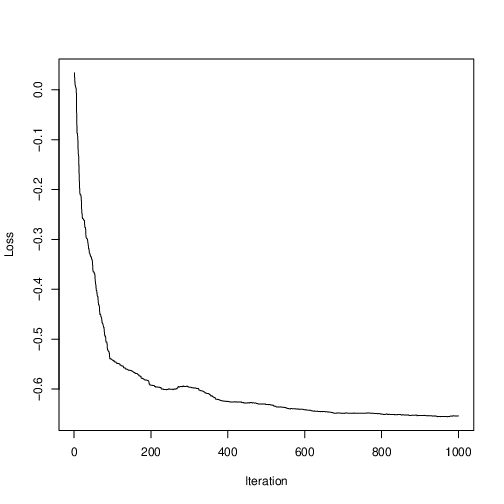
Figure 2 shows the loss values during the course of the optimization run; clearly some optimization has occurred, and progress has plateau’d. Being a stochastic optimization algorithm, it is not required to improve estimates at every iteration. In fact, Figure 2 shows that, for some iterations, loss increased. This is a healthy feature that enables SPSA to have a probability of bouncing out of inferior local optima, while an algorithm that is forced to take only steps that decrease loss would be highly likely to get stuck.
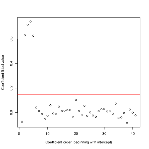
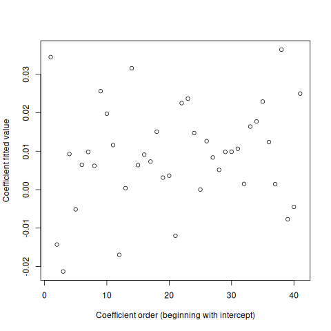
Figure 3 shows the coefficient estimates that minimize the loss. Among the coefficients, the first shown is the intercept term; the next four are the coefficients that are truly informative; the rest are purely noise, according to the simulation. The horizontal red line is a 3-SD threshold where I estimated the SD with a method robust to outliers (the hubers function in R’s MASS package). The optimization has perfectly identified which variables truly contribute.
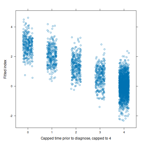
To clarify the behavior of the correlation metric for which the index is optimized, Figure 4 shows index values (with non-important variable coefficients set to zero) against capped time prior to diagnosis. Among all patients who are not diagnosed, this value is set to the cap, four. This is why many more points fall on four. The correlation coefficient (used in the loss function) for the plotted relationship is -0.866.
Assessing over-fitting
Why are the non-important coefficients in Figure 3 not estimated to be precisely zero? There are two possibilities.
First, SPSA is a first-order optimizer; it assumes local linearity. This can proceed towards an optimum point very quickly, but once the derivative-estimation gain constants span the optimum, the process is apt to bounce around near the optimum until the control sequences decay to zero. It’s like water spiraling down a drain; the water has reached the drain but can’t directly drop through it. A second-order process would estimate local curvature and, based on that, hop very close to the optimum point. Such an analog to SPSA exists but I haven’t tried it yet. Future work!
Also, SPSA is a stochastic optimizer. It makes random choices at every iteration. This can be very efficient. However, it means that at any given point in the process, if it has stopped making progress, we can’t be certain that it simply hasn’t yet found a path for improvement. With more and more iterations, such a possibility becomes less and less likely. But at any given moment, there is some uncertainty.
Second, it’s possible that small nonzero coefficients actually yield smaller loss than zero-valued coefficients. This would imply a degree of over-fitting.
The “best” value that SPSA found was -0.656, associated with many coefficients close to, but not equal to, zero. If we set the non-important coefficients all the way to zero, the loss is -0.657, 0.001 smaller. So there exists at least one parameter vector that beats the best that SPSA found (but we used SPSA to find it); if SPSA continued, it would converge to that value, or to a still-better one. We still can’t know if the absolute best sets coefficients to precisely zero. However, perfect can be the enemy of the good; we’ve solved our problem, because we’ve identified important variables and obtained good coefficients for them. Whether we zero out the remaining coefficients isn’t critical; for operational purposes at least, in most applications, we would do so.
I’ve repeated this exercise with both LASSO and ridge penalties, and with different penalty values, and these choices make little difference. The ridge penalty tends to move the four meaningful coefficient estimates closer together; this is typical behavior for the ridge penalty. It’s also optimizes more smoothly.
I’ve also tried optimizing with no penalty at all, and the optimization still leads to identical overall conclusions. However, I retained the small penalty weight of 0.01 out of principle.
Performance
Now let us calculate the identified linear combination using the four fitted coefficient values, setting the rest to zero, and applying the calculation to all observations from all subjects. Figure 1, shown in the introduction, shows traces for every subject in light gray. For the non-diagnosed subjects, the linear combination exhibits noise around zero at all time points. For the to-be-diagnosed subjects, at time -1.0 the linear combination is centered at zero with noise, and it grows linearly from there.
The apparent “bumpiness” at the five evaluated time points is an artifact of regression to the mean: values that happen to be in the extreme tails fail to repeat such at the next time point, giving what appears to be a saw-tooth pattern.
At some time point prior to diagnosis, a clinician should be able to monitor $$X\hat{\beta}$$ and at some time point he or she could confidently say that diagnosis is likely in the future. I’ll speak to that in a follow-up essay.
For the moment, please note that retrospectively identifying that the index is worth monitoring doesn’t address the specifics of how decisions based on the index would best be made.
The identified index could also be analyzed using other tools for longitudinal data, such as joint modeling, HMM’s, or generalized least squares. If analysis (rather than clinical monitoring) is the goal, Monitoring Regression could serve as a useful precursor to these inferential methods. Of course, using the same data twice—first to identify variables and fit an index, and second to do statistical analysis with a probabilistic model—introduces bias into the latter. A prospectively-gathered follow-up dataset is warranted.
The value of an index
Suppose we correctly identified that the first variable is important, but we only identified this one. Using this variable alone to monitor patients, we would see this analog of Figure 1:
The overall look is similar, and evidently there is some utility in monitoring, since the diagnosed patients show an upwards trend prior to the time of diagnosis. However, if we closely compare Figure 1 to Figure 5, we see that Figure 1 exhibits much better separation between non-diagnosed and diagnosed patients than does Figure 5. This accrues to Figure 1 being based on a synthesis (specifically a linear combination) of all four meaningful variables.
Negative example
The example above tests Monitoring Regression with known useful variables, and in that case it did well. Completeness demands that if a data set contains no useful variables, it should lead to a null conclusion.
Therefore I repeated the simulation as before—with 300 diagnosed patients, 300 undiagnosed patients, and 40 variables observed at each of five time points—except that all 40 variables are mean zero. No variable is informative. Nothing trends over time. Does my implementation of Monitoring Regression lead to the correct conclusion?
Happily, it does. Figure 6 shows estimated coefficients. They are all close to zero and none stand out; none exceed the robust 3-SD limit. While we don’t have a statistical inference to assure us, we can assess that the coefficients are small relative to the range of the variables. (In practice we should standardize all variables to ensure that we penalize coefficient magnitudes equally, so we could determine what makes a coefficient too small to be meaningful; I’ve neglected that here because I know all the variables have the same scale.)
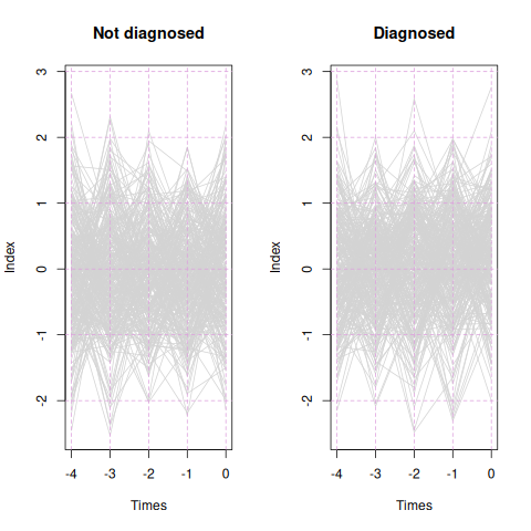
However, the real proof is whether the fitted index trends upwards for diagnosed patients and does nothing for undiagnosed patients. Figure 7 shows the patient traces. The diagnosed patients show no trend, just like the undiagnosed patients. The fitted index has no utility. Therefore we can be assured that if the data set has nothing happening, Monitoring Regression is unlikely to find something spurious.
Relation to Cox proportional hazard model with time-varying covariates
(This section is intended for a statistical audience.)
The astute statistical reader might ask whether Monitoring Regression is almost equivalent to the Cox proportional hazards model with time-varying covariates. The Cox model finds a linear combination of predictor variables that maximizes a concordance with outcome frequency.
More specifically, it divides time into intervals based on the times at which either an event occurred for some subject, or a subject left the study. Usually there are many such time points. (The fact that multiple intervals accrue from the same subject is ignored.) The Cox model treats the intervals essentially independently; one has a collection of intervals, each with its covariate values and its number of events, and based on that collection, a linear combination is sought which discriminates the intervals with more events from the intervals with fewer. With time-varying covariates, the covariate values within this collection of intervals may vary, even within subject. If the covariates do not vary over time, they may vary by subject, but are constant among intervals accruing from the same subject.
By default, the Cox model does not comprehend continuous change in covariates from previous time points. To add such effects, one can add lagged variables, or calculate change from earlier points.
In the simulation set-up used above, every subject is observed at each of 5 distinct and equal times. The only events that occur do so at the fifth time point. To identify covariate effects that predict risk of the event, the Cox model with time-varying covariates would evaluate covariate values at the fifth time point. An elevated value of x1, for instance, at the fifth time point, in a subject who is diagnosed, would tend to increase the coefficient value for an x1 effect. However, in that same patient, their x1 values may be elevated at the third and fourth time points, but since no diagnosis occurred then, these values tend to decrement the association of risk with elevated x1.
We could add lagged variables, or calculate change from the previous time. This would help a Cox model estimate that not only does x1 elevated at the fifth time increase risk, but that increase since the fourth time increases risk, and elevation at the fourth time point also adds to risk assessment.
However, similar data at earlier time points will partially mask these effects, since no events occurred at those times. In fact, the most effective Cox model would include all time points as lagged data at the final interval, in order to properly estimate risk as a function of a subject’s total trajectory. This would eliminate masking due to time intervals in which covariates are trending yet no event occurs. However, this would induce many problems:
- In typical use, we cannot count on having an equal number of time points per subject.
- The lagged model adds many variables, even though the goal of analysis is to find a set of variables worth monitoring using values available at the current time.
Monitoring Regression directs attention precisely at the monitoring problem and so is able to find a simple system. At every time point, Monitoring Regression uses only covariate values at that time. Trends are comprehended in the optimization metric rather than in the model itself. If one seeks a set of variables, and a function combining them, that uses only current-time values, yet is worth tracking over time, Monitoring Regression provides that directly.
Summary
Monitoring Regression takes a direct “model-free” approach to identifying variables that, in combination, can support monitoring to detect cases trending towards an event. I refer to “model-free” in quotes because the system does make some assumptions, which should be checked, but a probability distribution is not one of them. It could be a useful addition to the toolbox of any data analyst looking at sequential data with a monitoring perspective.